
Excel Name Ranges and Name Manager Overview
In this tutorial let’s talk about how to name groups of cells, tables, or even formulas in Excel, and how you can benefit from it.
For example, in this document, we have a group of cells that we want to rename as “Shortcuts”.
Let’s assign a name to this group of cells so you can see them in action. First, select the whole group either by manually selecting them or pressing CTRL+A

In the name box, on the upper left-hand corner of your spreadsheet you will see the Excel name box, right here, this is where the magic begins, at least for now.

Left click with your mouse inside the Name box until the text turns blue, then type the name Shortcuts and press ENTER

Important – When entering a name in this box:
- Start the name only with text or underscore _
- No spaces allowed, use an underscore _ instead
- Uppercase or lowercase are allowed
- Make it meaningful but as short as possible
- No special characters
- You can enter a number only after you enter the text
- Make sure that name is not used in a Worksheet or another name group
Examples of valid name formatting:

You can expand this field by placing your mouse under the three dots area and dragging it to the right.

What is the advantage of doing this extra step?
- This step can help you quickly locate frequently used data in your Workbook, think of it as bookmarks where you can easily click on, and it will take you to that named group even if the group is in another worksheet or “page” within the same workbook.
Where can we edit, delete, and add comments if needed to each named range?
- The Excel Name Manager was the answer! In here we can edit, delete, filter, add comments and so much more, there are some amazing things hidden in this little tool right here.
- To get there click on the Formulas Tab and under Defined Names group, select the Name Manager Tool

Another shortcut to get here is CTRL+F3, depending on your computer you may want to try Function (fn on your keyboard) + F3
How to Edit a Name and add a comment in the Excel Name Manager?
First, click on the Name Manager, the following box appears.
- You can sort alphabetically by clicking on the Name Column Header
- Double-click on the name you wish to change.
- For this example, we are double clicking “Shortcuts”

- The Edit section appears, we will change the name from “Shortcuts” to “Excel_Shortcuts” by re-typing it, to make it more meaningful. Note that we use the underscore instead of a space.
- Notice that we also added the comment to help other users not to delete in this case.
- Click OK to Save your changes.

How to Delete a Name using the Excel Name Manager?
In the Name Manager Area, you can select the Name of your choice, highlighted in blue and press the “Delete” button.
By doing this step, you will not delete the data inside that name range, only its group name or “bookmark” attribute.

To confirm your deletion, the message “Are You sure you want to delete the name First_Day? Press OK to save your changes.

What else can we do inside the Name Manager in Excel?
- Aside from the awesome “bookmarking” features, we discovered some other hidden tools:
- Use the Excel Name Manager Filters
- Clear filter
- Names Scoped to Worksheet: These are names only visible inside a specific worksheet
- Names Scoped to Workbook: This is the default (and what you may want) so you can access the entire workbook.

- Names with / without Errors : helps you spot the names with errors like the example below. A separate tutorial on how to repair these and other formula, function and calculation errors will be released soon, so we can go deep into this.

Use the name range inside a formula
We renamed the following table of insurance policies Table as “Ins_List” in Excel
Let’s use the name in two Vlookups, one that will help me get the Agent name of any policy number
The second Vlookup will help me get the state of the policy

Under the Agent Box type =Vlookup(L5, and here you can go to the Use in Formula dropdown, click the Ins_List table and continue typing the rest of the values, remember to close parenthesis until the formula looks like this:
=VLOOKUP(L5,Ins_List,4,FALSE)
You should see the Agent Rebecca in your results

Repeat the steps under the State white box, until the formula looks like this:
Tip: col_index_num is 9 because what we are looking for the State in the ninth column

Double check the results to see if they are accurate and that is another way to use the name ranges


How to export the Paste the list of your name range
This last method will help you review in a separate Worksheet the contents of your “bookmarks” or Named list.
Warning: This is not your typical Excel copy/paste, as the list will be connected to its source, we’ll show you in a bit what we mean.
Let’s say that you need to review separately the list of the Ins_List table
Click on the cell where you want the results to be paste to in the new Sheet, we picked B2
Tip: always make sure it won’t overlap any existing data if you are not using a blank Sheet.

Open a new Worksheet >> Go to the Formulas Tab >> Name Manager
This time we will select “Use in Formula” and scroll down and click on “Paste List”
Click on the Ins_List until blue and then OK

Tip: Do not click “Paste List” here, or you will see this instead:

If you see the = sign followed by the Name you are in the right track, press Enter

After pressing enter, the information from the list is also in the new Sheet

This is not your typical copy/paste
Any Edits you make though need to be done from the original table and not here, or you will have a #spill error, press CTRL+Z if this happens to revert back.
To work around this issue, you can select the whole table from here with CTRL+A, copy and paste its values only in a separate column and then delete the initial list like this.

We hope you enjoyed our tutorial please don’t forget to like and subscribe to our channel and help us create more free content about technology here.
Excel Name Ranges and Name Manager Overview
In this tutorial let’s talk about how to name groups of cells, tables or even formulas in Excel, and how you can benefit from it.
For example, in this document we have a group of cells that we want to rename as “Shortcuts”.
Let’s assign a name to this group of cells so you can see them in action. First select the whole group either by manually selecting them or pressing CTRL+A

In the name box, on the upper left-hand corner of your spreadsheet you will see the Excel name box, right here, this is where the magic begins, at least for now.

Left click with your mouse inside the Name box until the text turns blue, then type the name Shortcuts and press ENTER

Important – When entering a name in this box:
- Start the name only with text or underscore _
- No spaces allowed, use an underscore _ instead
- Uppercase or lowercase are allowed
- Make it meaningful but as short as possible
- No special characters
- You can enter a number only after you enter the text
- Make sure that name is not used in a Worksheet or another name group
Examples of valid name formatting:

You can expand this field by placing your mouse under the three dots area and dragging it to the right.

What is the advantage of doing this extra step?
- This step can help you quickly locate frequently used data in your Workbook, think of it as bookmarks where you can easily click on, and it will take you to that named group even if the group is in another worksheet or “page” within the same workbook.
Where can we edit, delete, and add comments if needed to each named range?
- The Excel Name Manager was the answer! In here we can edit, delete, filter, add comments and so much more, there are some amazing things hidden in this little tool right here.
- To get there click on the Formulas Tab and under Defined Names group, select the Name Manager Tool

Another shortcut to get here is CTRL+F3, depending on your computer you may want to try Function (fn on your keyboard) + F3
How to Edit a Name and add a comment in the Excel Name Manager?
First, click on the Name Manager, the following box appears.
- You can sort alphabetically by clicking on the Name Column Header
- Double-click on the name you wish to change.
- For this example, we are double clicking “Shortcuts”

- The Edit section appears, we will change the name from “Shortcuts” to “Excel_Shortcuts” by re-typing it, to make it more meaningful. Note that we use the underscore instead of a space.
- Notice that we also added the comment to help other users not to delete in this case.
- Click OK to Save your changes.

How to Delete a Name using the Excel Name Manager?
In the Name Manager Area, you can select the Name of your choice, highlighted in blue and press the “Delete” button.
By doing this step, you will not delete the data inside that name range, only its group name or “bookmark” attribute.

To confirm your deletion, the message “Are You sure you want to delete the name First_Day? Press OK to save your changes.

[You can watch the full video here]
What else can we do inside the Name Manager in Excel?
- Aside from the awesome “bookmarking” features, we discovered some other hidden tools:
- Use the Excel Name Manager Filters
- Clear filter
- Names Scoped to Worksheet: These are names only visible inside a specific worksheet
- Names Scoped to Workbook: This is the default (and what you may want) so you can access the entire workbook.

- Names with / without Errors : helps you spot the names with errors like the example below. A separate tutorial on how to repair these and other formula, function and calculation errors will be released soon, so we can go deep into this.

Use the name range inside a formula
We renamed the following table of insurance policies Table as “Ins_List” in Excel
Let’s use the name in two Vlookups, one that will help me get the Agent name of any policy number
The second Vlookup will help me get the state of the policy

Under the Agent Box type =Vlookup(L5, and here you can go to the Use in Formula dropdown, click the Ins_List table and continue typing the rest of the values, remember to close parenthesis until the formula looks like this:
=VLOOKUP(L5,Ins_List,4,FALSE)
You should see the Agent Rebecca in your results

Repeat the steps under the State white box, until the formula looks like this:
Tip: col_index_num is 9 because what we are looking for the State in the ninth column

Double check the results to see if they are accurate and that is another way to use the name ranges

How to export the Paste the list of your name range
This last method will help you review in a separate Worksheet the contents of your “bookmarks” or Named list.
Warning: This is not your typical Excel copy/paste, as the list will be connected to its source, we’ll show you in a bit what we mean.
Let’s say that you need to review separately the list of the Ins_List table
Click on the cell where you want the results to be paste to in the new Sheet, we picked B2
Tip: always make sure it won’t overlap any existing data if you are not using a blank Sheet.

Open a new Worksheet >> Go to the Formulas Tab >> Name Manager
This time we will select “Use in Formula” and scroll down and click on “Paste List”
Click on the Ins_List until blue and then OK

Tip: Do not click “Paste List” here, or you will see this instead:

If you see the = sign followed by the Name you are in the right track, press Enter

After pressing enter, the information from the list is also in the new Sheet

This is not your typical copy/paste
Any Edits you make though need to be done from the original table and not here, or you will have a #spill error, press CTRL+Z if this happens to revert back.
To work around this issue, you can select the whole table from here with CTRL+A, copy and paste its values only in a separate column and then delete the initial list like this.

We hope you enjoyed our tutorial please don’t forget to like and subscribe to our channel and help us create more free content about technology here.
Excel Name Ranges and Name Manager Overview
In this tutorial let’s talk about how to name groups of cells, tables, or even formulas in Excel, and how you can benefit from it.
For example, in this document, we have a group of cells that we want to rename as “Shortcuts”.
Let’s assign a name to this group of cells so you can see them in action. First, select the whole group either by manually selecting them or pressing CTRL+A

In the name box, on the upper left-hand corner of your spreadsheet, you will see the Excel name box, right here, this is where the magic begins, at least for now.

Left click with your mouse inside the Name box until the text turns blue, then type the name Shortcuts and press ENTER

Important – When entering a name in this box:
- Start the name only with text or underscore _
- No spaces allowed, use an underscore _ instead
- Uppercase or lowercase are allowed
- Make it meaningful but as short as possible
- No special characters
- You can enter a number only after you enter the text
- Make sure that name is not used in a Worksheet or another name group
Examples of valid name formatting:

You can expand this field by placing your mouse under the three dots area and dragging it to the right.

What is the advantage of doing this extra step?
- This step can help you quickly locate frequently used data in your Workbook, think of it as bookmarks where you can easily click on, and it will take you to that named group even if the group is in another worksheet or “page” within the same workbook.
Where can we edit, delete, and add comments if needed to each named range?
- The Excel Name Manager was the answer! In here we can edit, delete, filter, add comments and so much more, there are some amazing things hidden in this little tool right here.
- To get there click on the Formulas Tab and under Defined Names group, select the Name Manager Tool

Another shortcut to get here is CTRL+F3, depending on your computer you may want to try Function (fn on your keyboard) + F3
How to Edit a Name and add a comment in the Excel Name Manager?
First, click on the Name Manager, the following box appears.
- You can sort alphabetically by clicking on the Name Column Header
- Double-click on the name you wish to change.
- For this example, we are double clicking “Shortcuts”

- The Edit section appears, we will change the name from “Shortcuts” to “Excel_Shortcuts” by re-typing it, to make it more meaningful. Note that we use the underscore instead of a space.
- Notice that we also added the comment to help other users not to delete in this case.
- Click OK to Save your changes.

How to Delete a Name using the Excel Name Manager?
In the Name Manager Area, you can select the Name of your choice, highlighted in blue and press the “Delete” button.
By doing this step, you will not delete the data inside that name range, only its group name or “bookmark” attribute.

To confirm your deletion, the message “Are You sure you want to delete the name First_Day? Press OK to save your changes.

[You can watch the full video here]
What else can we do inside the Name Manager in Excel?
- Aside from the awesome “bookmarking” features, we discovered some other hidden tools:
- Use the Excel Name Manager Filters
- Clear filter
- Names Scoped to Worksheet: These are names only visible inside a specific worksheet
- Names Scoped to Workbook: This is the default (and what you may want) so you can access the entire workbook.

- Names with / without Errors : helps you spot the names with errors like the example below. A separate tutorial on how to repair these and other formula, function and calculation errors will be released soon, so we can go deep into this.

Use the name range inside a formula
We renamed the following table of insurance policies Table as “Ins_List” in Excel
Let’s use the name in two Vlookups, one that will help me get the Agent name of any policy number
The second Vlookup will help me get the state of the policy

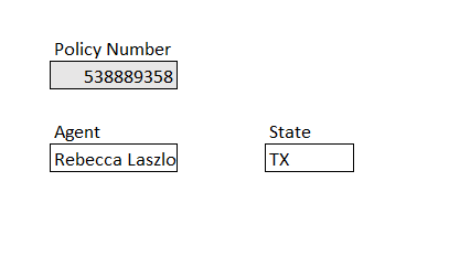
Under the Agent Box type =Vlookup(L5, and here you can go to the Use in Formula dropdown, click the Ins_List table and continue typing the rest of the values, remember to close parenthesis until the formula looks like this:
=VLOOKUP(L5,Ins_List,4,FALSE)
You should see the Agent Rebecca in your results

Repeat the steps under the State white box, until the formula looks like this:
Tip: col_index_num is 9 because what we are looking for the State in the ninth column

Double check the results to see if they are accurate and that is another way to use the name ranges


How to export the Paste the list of your name range
This last method will help you review in a separate Worksheet the contents of your “bookmarks” or Named list.
Warning: This is not your typical Excel copy/paste, as the list will be connected to its source, we’ll show you in a bit what we mean.
Let’s say that you need to review the list of the Ins_List table separately
Click on the cell where you want the results to be paste to in the new Sheet, we picked B2
Tip: always make sure it won’t overlap any existing data if you are not using a blank Sheet.

Open a new Worksheet >> Go to the Formulas Tab >> Name Manager
This time we will select “Use in Formula” and scroll down and click on “Paste List”
Click on the Ins_List until blue and then OK

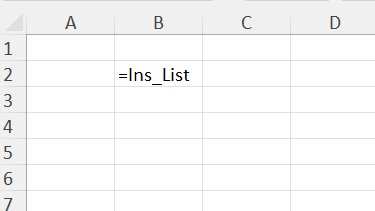
Tip: Do not click “Paste List” here, or you will see this instead:

If you see the = sign followed by the Name you are in the right track, press Enter
After pressing enter, the information from the list is also in the new Sheet

This is not your typical copy/paste
Any Edits you make though need to be done from the original table and not here, or you will have a #spill error, press CTRL+Z if this happens to revert back.
To work around this issue, you can select the whole table from here with CTRL+A, copy and paste its values only in a separate column and then delete the initial list like this.

We hope you enjoyed our tutorial please don’t forget to like and subscribe to our channel and help us create more free content about technology here.
Link: https://www.youtube.com/c/iKnowledgeSchool?sub_confirmation=1
Excel name ranges
How to name ranges in Excel
How to use the name manager in Excel
How to name a cell in Excel